From Apples to Strawberries

Two weeks ago, OpenAI released the o1 series.

This publicly marks the start of the “search” paradigm in modern ML, just as ChatGPT’s launch in 2022 marked the arrival of the “learning” paradigm. 

With this new paradigm, you should expect progress in ML performance over the next two years to be at least as fast as it was in the last two years. In fact, there are reasons to expect it to be even faster.

Here’s why!

Bitter lesson 2: electric boogaloo

When I talk about “learning” and “search”, I mean the two “general methods that leverage computation” which Rich Sutton named in The Bitter Lesson. Loosely, “learning” is fitting to patterns in the world, while “search” is finding the best option in a space of possibilities.

The Bitter Lesson explains why a single model launch, like o1’s, can catalyse such rapid progress. Since “the most effective” methods in ML are these general methods, progress in ML doesn’t occur steadily, but instead comes in fits and spurts. This is because it relies on researchers finding a technique which gets predictably better with more computing power (“compute”). Once they have conviction in it, they can scale that technique with more compute. A model launch is simply a lagging indicator of this conviction.

With “learning”, some researchers had the realisation in 2020 that they could use more compute to train a model with more parameters on more data, and it would just improve. Thus they spent the next two years doing that, and in the process, learnt a lot about how to use that compute effectively. This unlocked ChatGPT in 2022, and has continued to power the last two years of improvements in AI.

(Check out yesterday’s post if you’re curious about how this came to pass!)

Moving from training to inference

However, most of this compute has been used during the training process of the models. This is a result of how “learning” works. If you want the model to learn more during training, you can scale that pretty arbitrarily, just by making it bigger or having it see more data. By contrast, the model can only learn during inference if you give it in-context examples, but this is constrained by the size of its context window, which isn’t infinitely scalable.

This means that spending more compute on inference was always the next frontier to be tackled. Many users of these models have tried to do clever prompting or build convoluted wrappers around these models to take advantage of that. You may have heard of techniques like “in-context learning”, “chain of thought” and so on.

This is a mistake.

By handcrafting these scaffolds, they are ignoring The Bitter Lesson at their own peril. What they needed to do instead was to find a method that could scalably absorb compute at inference time, without their intervention. Many researchers at top AI labs have long suspected that “search” fits this description:

• Noam Brown (July 2023): “I’ll now investigate how to make these [self-play and reasoning] methods truly general”
• The Information (November 2023): “among the techniques the [OpenAI] team experimented with was … test-time computation”
• Dwarkesh Patel (December 2023): “almost all the researchers I talk to in the big AI labs are quite confident they’ll get self-play to work”

The basic idea behind “search” is that you can solve hard problems by trying many different paths and seeing which gets you the best outcome. Since you can try arbitrarily many paths if you’re willing to spend the compute, this is something that can pretty naturally scale at inference time.

Verification is easier than generation

There’s a long history of “search” working in other domains. One notable example is AlphaGo Zero, which was DeepMind’s system for playing Go. This system had two parts: a neural network and a Monte Carlo Tree Search algorithm.

The neural net generates:

• An estimate of how good the current board state is
• The probability of different next moves given the current board state

The MCTS algorithm looks at all possible next moves and picks a move. Early in the game, it tries to pick moves it hasn’t encountered yet. As it becomes more certain about which move is good or bad, it focuses on picking the best possible move. Essentially, it’s trying to sensibly trade off “exploration” and “exploitation”. After the MCTS algorithm has picked a move, the neural net evaluates the board state conditional on that move being made and updates the algorithm’s knowledge of how good each move is.

To improve this system, they got it to play against itself. At the end of each game, the self-play produced a series of data about what the board state was after each move, what the MCTS algorithm thought it should do and who ended up winning the game. This data could then be used to train the neural network, making it better and better each time. 

At inference, the combination of the trained neural net and the MCTS algorithm produced the superhuman performance of AlphaGo Zero system. This was rated at over 1000 Elo points above the AlphaGo Lee system that had famously beat Lee Sedol.

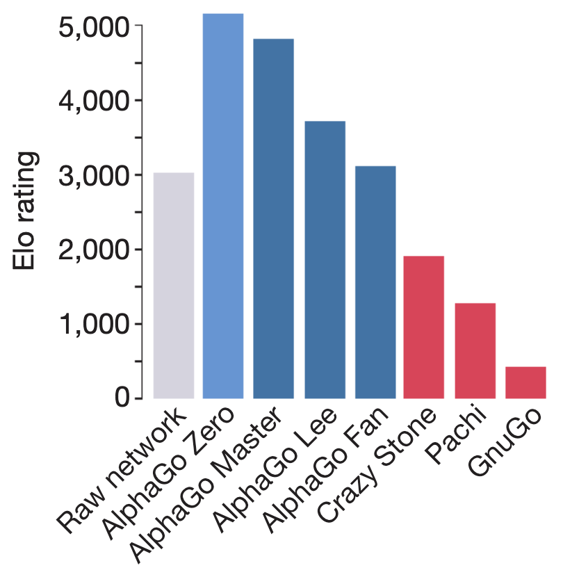
Notice that search is key!

When doing inference without MCTS (“raw network”), it was over 2000 Elo points below the version with MCTS, and actually underperformed even AlphaGo Lee. In fact, if we wanted to bridge the gap between the raw network and the network with MCTS, but without doing any search, the neural network would need to be 100,000x bigger.

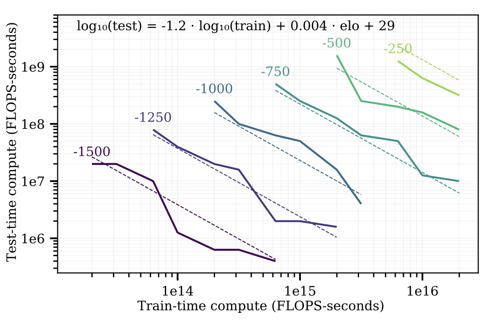
This training-inference trade-off is replicated across other games. For example, Jones found that you can attain the same Elo in Hex on a model with 10x less training compute by spending 15x on inference compute:

In general, the “search” process follows a certain loop:

1. Get the model to play against itself
2. Break down the “play” into steps
3. Have a search algorithm explore over the steps
4. Verify if the end result was good
5. Tell the search algorithm so it learns which steps are good
6. Train the model based on what the search algorithm has learnt

In the case of games like Go and Hex, the existence of pre-defined rules, moves and win conditions mean that this loop is pretty easy to do. However, what about domains that are less well specified?

Combining learning and search

To start with, researchers have focused on fields like mathematics or coding, where it is possible to do verification to some degree e.g. with theorem provers or unit tests. Much of the exciting research in the past two years has been about bringing “search” to these areas.

The simplest version of “search” is one step deep. That means doing many single step generations and then picking the best one. One way of picking is to take the most popular answer. It’s a bit like the “Ask the Audience” lifeline on “Who Wants To Be A Millionaire”!

This is the majority voting approach from Lewkowycz et al., and doing so (“maj1@k”) with the Minerva model shows dramatic improvements relative to just using model itself across STEM benchmarks:

	MATH	GSM8K	MMLU-STEM
Minerva (540B)	33.6%	58.8%	63.9%
Minerva (540B), maj1@k	50.3%	78.5%	75.0%

A more sophisticated approach is to swap about majority voting for a neural network that tries to pick the best answer. This is known as an “outcome reward model”, and Lightman et al. find that doing this improves their results on the MATH benchmark from 69.6% accuracy with majority voting to 72.4%.

To make it even better, they break down the problem into multiple steps, and train a “process reward model”. This model looks at every step of the reasoning process, instead of just the output, and picking the answer using this model brings accuracy to 78.2%.

This is shaping up to a similar loop as before:

1. Get the language model to respond to a prompt
2. Each “move” is the model generating some reasoning steps
3. A search algorithm picks whether to keep taking more “moves”
4. Verify if the eventual answer is correct
5. Tell the search algorithm so it learns which “moves” were good
6. Train the model based on what the search algorithm has learnt

By repeating this many times per prompt for billions of prompts, you get a language model that is much better at generating reasoning steps, as well as a search algorithm that knows if a particular set of reasoning steps is good. At inference, you can use this by generating some reasoning steps, and then either re-generating it or taking the next set of reasoning steps, depending on whether the search algorithm thinks this was a good “move”.

Then you can scale this in two ways: by spending more time on training compute (e.g. more prompts, more attempts per prompt) or by spending more time on inference compute (e.g. setting a higher threshold for what a good “move” is, trying many “moves”).

Scaling laws, redux

This is an interesting hypothesis. Does it actually let us scale inference compute though?

Here are a few reasons it might not:

1. Maybe none of the “moves” are good enough i.e. if you asked a 3 year old an advanced college maths question, it doesn’t matter how many times you ask them and how well you can search through their answers: they simply aren’t smart enough
2. Maybe verification is hard enough that the search algorithm doesn’t learn much and can’t help us
3. Even if the first two aren’t completely true, they may be true enough that it is not economical to use inference compute, relative to training compute

Let’s tackle each in order.

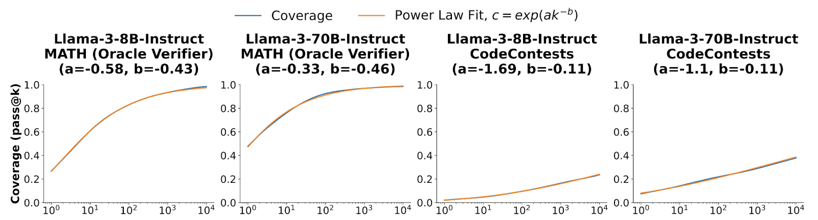
It’s not super surprising that if you do more sampling, the probability that at least one of the samples will be the correct answer (“coverage”) increases, at least a little bit. What Brown et al. show us is that this scales to an unbelievable degree (i.e. to tens of thousands of samples) and scales following a predictable power law:

By simply sampling many times and picking the answer based on an automated verifier, this increase in “coverage” translates directly into better performance. In fact, they manage to beat the state-of-the-art SWE-bench Lite results by a staggering 13pp (and as of this post, would still top the leaderboard):

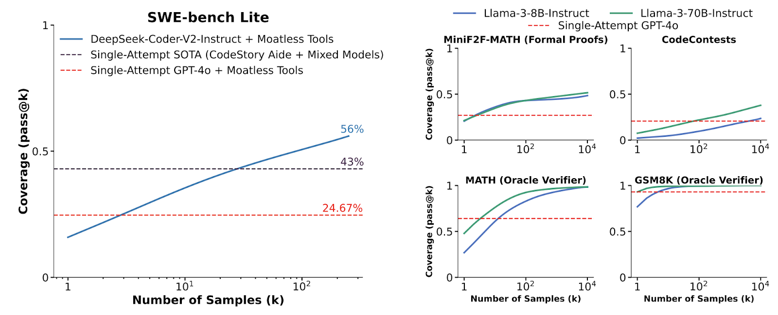
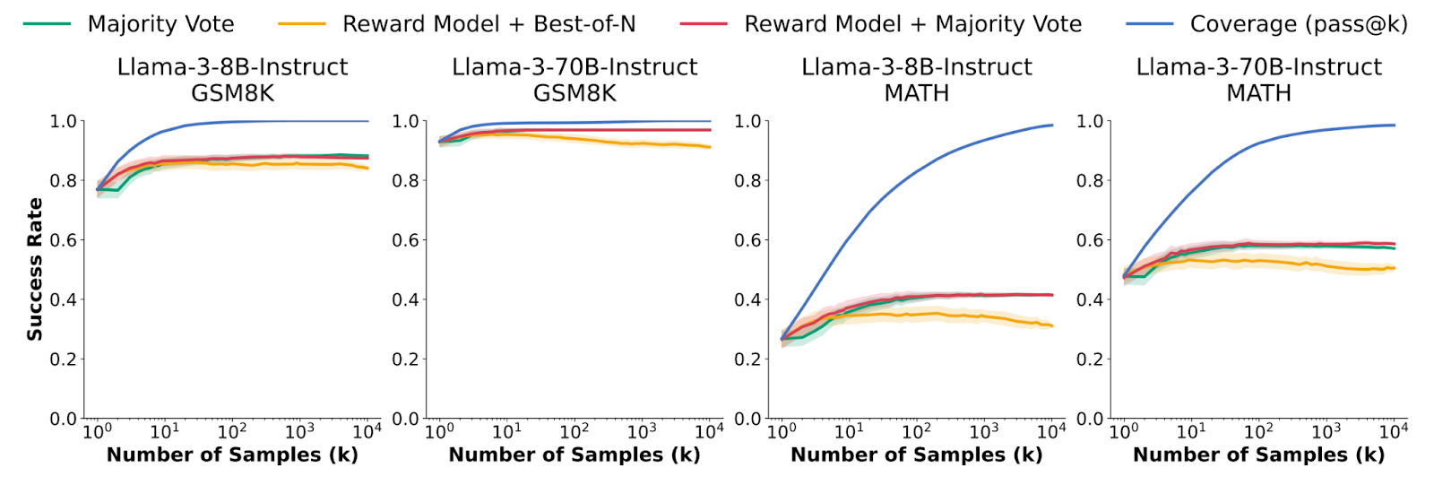
Thus, issue 1 isn’t a problem. However, they also show that for maths problems without theorem provers, verification isn’t that easy. Whether it is with majority voting or using a reward model to search over the samples, it seems that this plateaus quickly, causing a gap between “coverage” and the actual success rate:

This means that issue 2 is only half-solved, for certain domains with easy verifiers. What does this mean for issue 3 i.e. trading off training and inference compute?

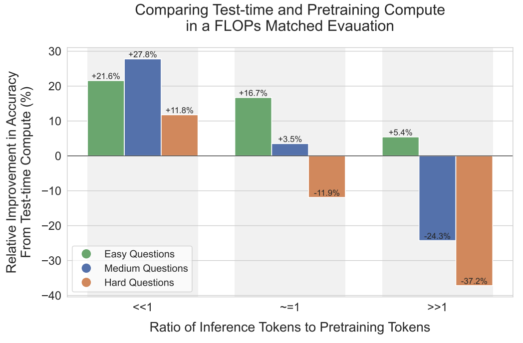
This is where Snell et al. come in. They ask the question: “if you can 10x the combined amount of training and inference compute, how much should you spend on each?”. They find that the two types of compute are substitutable, but not perfectly, and inference compute is best spent on easier problems.

The unhobbling is coming  

Let’s take a step back.

Long before ChatGPT came out, and before even OpenAI existed, Ilya Sutskever had said that “the models, they just want to learn”. The belief that you could pour more training compute and scale up “learning” is not a new one. Yet it took ChatGPT to turn it into a public and undeniable fact.

For the past two years, we have been in the pre-ChatGPT era with “search”. While all of the research I’ve mentioned above kept pointing in the direction of scaling inference compute, no one had productionised and done it in a way that made it public and undeniable.

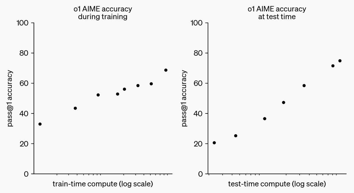
On September 12th, o1 changed that:

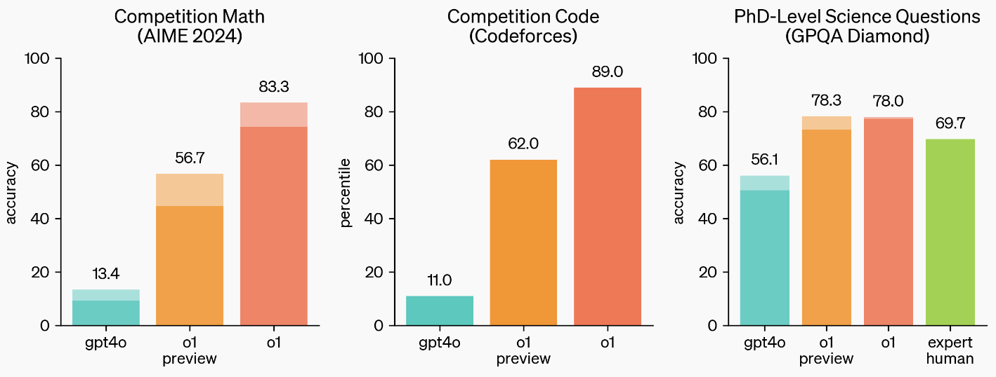
By themselves, these results on competition mathematics and coding problems are already impressive. These are hard problems where o1 blows GPT-4o out of the water, but in some ways, this can be expected, since maths and code can have very good verifiers that provide a clear reward signal to the search algorithm.

What is more staggering is the performance on other domains:

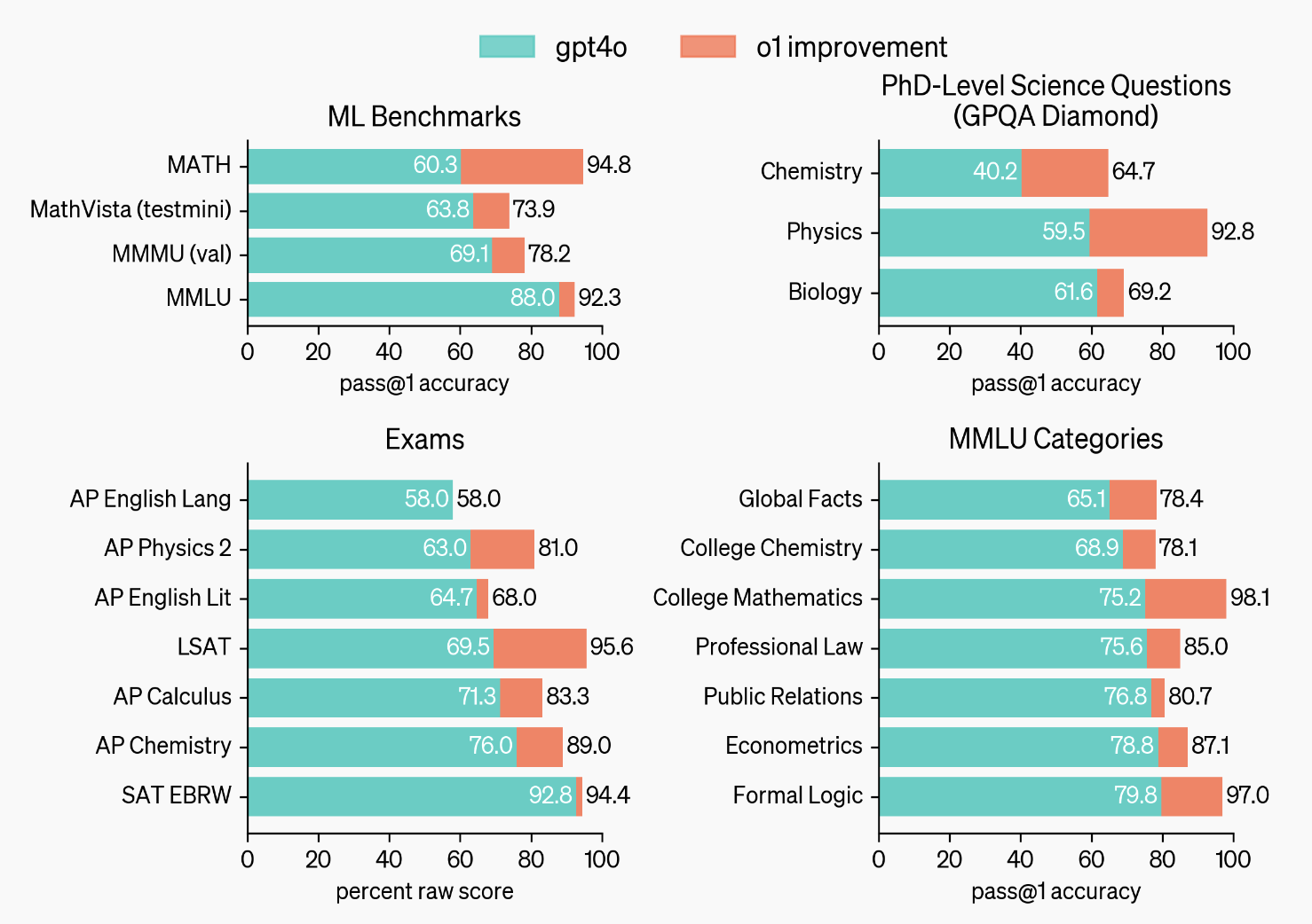
For example, GPQA is a “Google-proof” science benchmark that even domain PhDs struggle with, and yet o1 beats them and gpt-4o very handily. Nor is this limited to STEM: o1 also improves on gpt-4o’s performance on the LSATs, econometrics etc. 

In addition to validating how search can work on more general domains, o1 also shows that it can scale, across both training and inference compute:

Just as ChatGPT fired the starting gun for the race to scale “learning”, o1 has done the same for “search”!

Why does this matter?

Scaling “search” on its own will improve domain-specific capabilities. Instead of needing to re-train a model, you can simulate what a larger model’s performance would be by simply spending more inference compute to solve your problem. This pulls forward the ability to deploy AI systems into real world problems, and makes the price-performance trade-off less discontinuous and dependent on research labs releasing new models.

Just to give a sense of price, Zhang’s replication of the scaling plot lets us estimate that the maximum accuracy displayed can be achieved with $1.6 of inference compute per problem. That’s almost certainly cheaper than how much it would have cost to train a model that gets the same accuracy without “search”.

This alone would make scaling “search” as exciting as scaling “learning” has been. However, it turns out that "search" will also make "learning" better.

Already, lots of training data is synthetic i.e. generated by an AI. Now, every single set of reasoning steps by o1 can be used to train the next model. Since o1 is smarter, the quality of these reasoning traces is higher, and it can filter out the bad sets of reasoning steps better than before.

The reason we couldn’t make this data flywheel in the past is because the models weren’t smart enough to generate useful reasoning traces, or filter out the bad ones. Now that we seem to have reached that threshold, we can follow the same playbook which made AlphaGo superhuman: bootstrapping the next model from the outputs of the previous one.

That’s why Sam Altman is so confident that “deep learning worked”, and why you should expect even faster progress soon. Remember, the models are the worst they’ll ever be!

Thanks to Kevin Niechen, Zhengdong Wang, Jannik Schilling, Bradley Hsu, Devansh Pandey, Zach Mazlish and Basil Halperin for discussion and feedback.