Three Kuhnian Revolutions in ML Training

Parameters and data.

These are the two ingredients of training ML models. The total amount of computation (“compute”) you need to do to train a model is proportional to the number of parameters multiplied by the amount of data (measured in “tokens”).

Four years ago, it was well-known that if you had more compute to train a model, you should spend most of it on parameters.

Two years ago, everyone changed their mind and believed you should spend it equally on parameters and data.

Just last year, it became widely accepted that you should spend orders-of-magnitude more on data than anyone had previously thought.

Why have the recipes to training these models changed so much, and so frequently? To understand this, we need to take a walk through the intellectual history of scaling modern ML models.

The Bitter Lesson

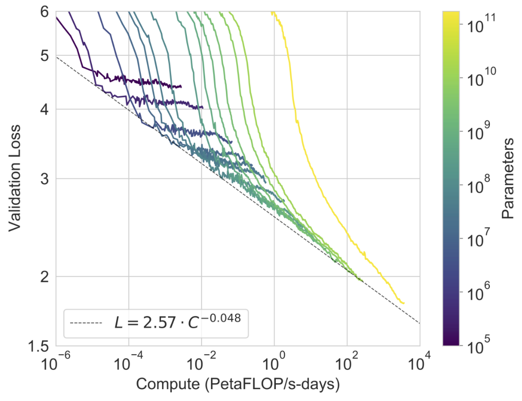
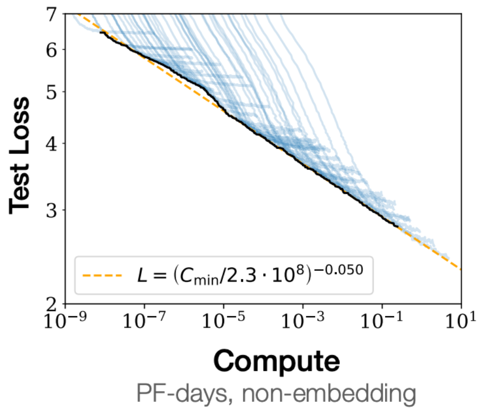
The science of training large models starts with Kaplan et al. in early 2020. In the paper, the OpenAI team tested different configurations of transformer language models. The two most important axes they varied were the number of model parameters (768 to 1.5B) and number of tokens in the dataset (22M to 23B). Implicitly, this also varied the total amount of compute used to train the model, since compute ~ parameters x tokens.

They found a stable and predictable power-law relationship between compute and the performance of the model. Here, performance is measured by the “loss”, which is simply the model’s error in predicting the next token across all the text it is trained on:

They also gave a formula for how to use your compute efficiently, since for any fixed amount of compute, there is a trade-off between making the model bigger and training it on more data. Kaplan showed that if you could 10x the amount of compute, you should 5x the number of parameters and 2x the number of tokens it is trained on.

The punchline was that 5 months later, the OpenAI team launched GPT-3. With a staggering 175B parameters trained on 300B tokens, this validated the Kaplan scaling laws with three orders of magnitude more compute than the biggest Kaplan model:

With GPT-3, OpenAI had demonstrated that the scaling law was really quite predictable. While “bigger is better” wasn’t the most surprising result, the idea that you could predict exactly how good it would be, and could get a recipe for the exact ratio of parameters-to-tokens was unprecedented.

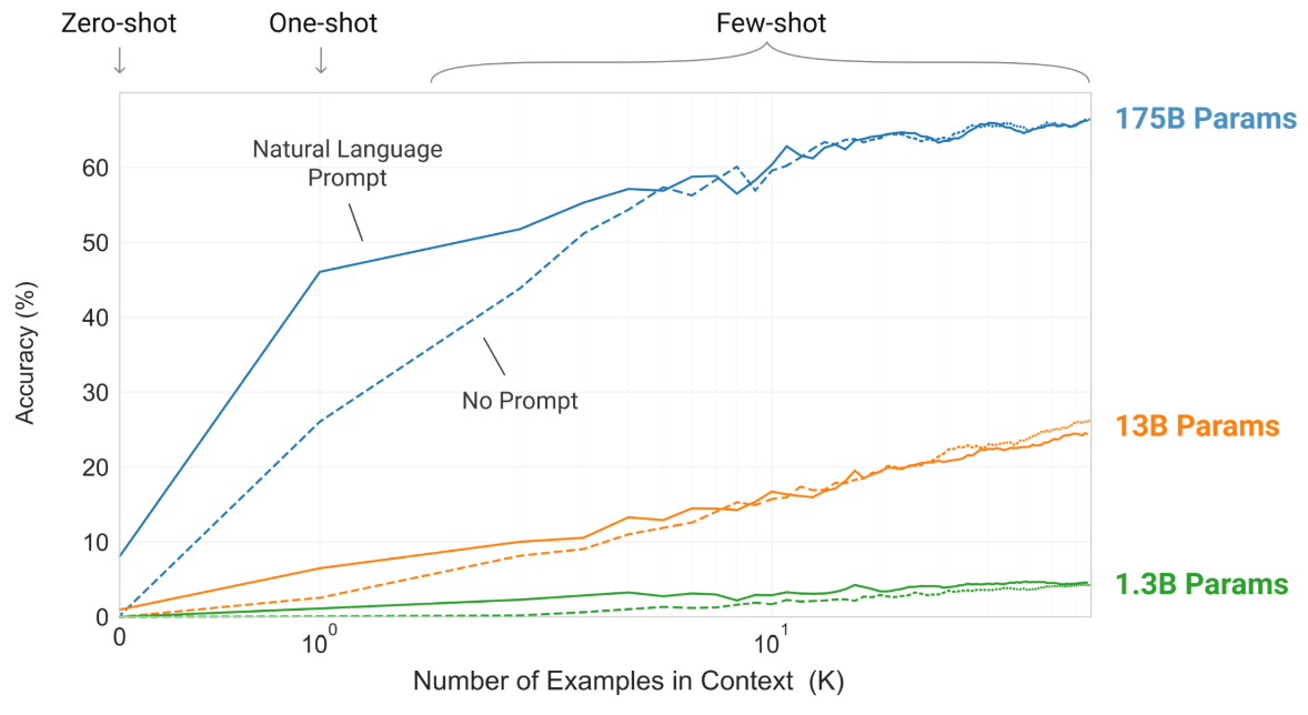
They had also shown that size was qualitatively important: while the “loss” of the model changed steadily with size, the actual human-relevant capabilities were more discontinuous and emerged above certain thresholds. One “emergent capability” was the ability for models to reason in-context i.e. learn how to do a task accurately if you gave it one (“one-shot”) or multiple (“few-shot”) examples. By being given examples, large models gained a lot more accuracy than smaller models:

After an initial period of shock, everyone quickly followed suit: DeepMind released Gopher (280B parameters, 300B tokens) in late 2021 and NVIDIA released Megatron (530B parameters, 270B tokens) in early 2022.

Chinchilla outperforms Gopher

Yet just as the race to train big models was heating up, it would get interrupted in March 2022 by Hoffmann et al., better known as the Chinchilla scaling laws. In this paper, the DeepMind team revisited what the right ratio of parameters to tokens was for any fixed amount of compute. What they found was that data was far more important than people realised!

They took three approaches to this, but the second “isoFLOP” method is most intuitive:

• Take a fixed amount of compute
• Pick a range of model sizes where the larger ones will be trained on less data
• Plot each model’s performance against parameters and join the dots to get an isoFLOP curve, where each point has the same total compute
• The lowest point on the curve has the best performance

The Chinchilla team exhaustively trained over 400 models across 9 different isoFLOP curves:

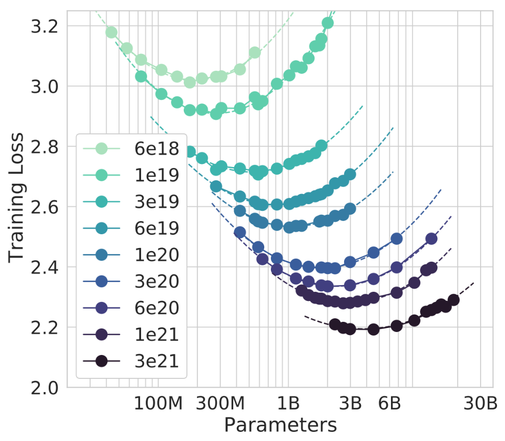
By fitting a regression line to the minimum point of each isoFLOP curve, they found that a 10x increase in compute should be split equally between model size and dataset size i.e. 3.1x each of them, rather than Kaplan’s 5x and 2x split.

As with Kaplan, they validated this by training a model with even more compute than their experiments. In particular, they took Gopher’s FLOP count but trained it with the parameter-token split implied by their experiments. This was “Chinchilla”! With 70B parameters trained on 1.4T tokens, it blew past Gopher on every single benchmark e.g. the Pile, MMLU, BIG-Bench etc.

What did Kaplan get wrong?

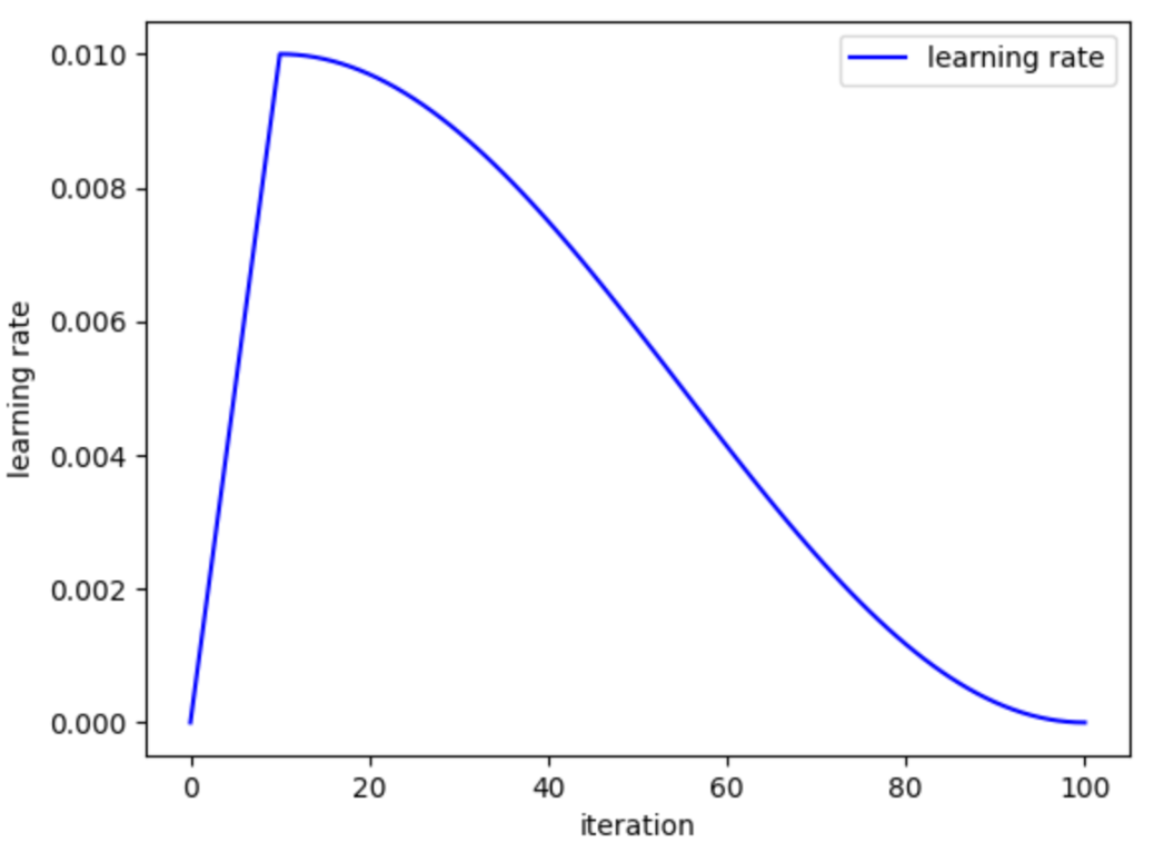
The immediate difference between the two papers was the choice of the learning rate schedule. The learning rate determines how much the parameters of a model change when it sees each token of training data. A common LR schedule is to start training with a low LR and build it up linearly to let the model “warm up”, and then slowly decay from the maximum across the rest of training:

Kaplan had picked a LR schedule with 3000 steps of warmup followed by a fixed decay schedule. When Chinchilla first came out, they suggested that Kaplan’s problem was having the same LR schedule for every model, rather than matching the length of the decay to the amount of data the model was trained on.

In the past few months, however, new work from Porian et al. has suggested that there might be more at play. By recreating the Kaplan experiments, they found that Chinchilla’s hypothesis about LR decay wasn’t that important. What mattered more was:

• Kaplan ignoring the compute used by last layer of the model
• Kaplan’s fixed 3000 steps of warmup (which meant smaller models trained on less data spent relatively more time in warmup)
• Kaplan using the same hyperparameters for all model sizes, rather than tuning them for each one

All of this to say, the science of scaling is still pretty nascent! Regardless, one thing is clear: Chinchilla’s recipe set the bar for how to train large language models. Since then, every time someone says they are training a “compute optimal model”, they mean that they are following Chinchilla when deciding the parameter-token split.

Llama outperforms Chinchilla

Unfortunately, the description “compute optimal” ended up being rather misleading, even to researchers in the field. That’s because what Chinchilla means by “compute optimal” is “training compute optimal” i.e. the best parameter-token split if you only consider the compute you spend in training the model. However, you will also want to serve the model for inference, and larger models cost more to serve. Thus very rarely, if ever, do you actually want to train a Chinchilla optimal model.

Instead, you want to train on fewer parameters but more tokens i.e. moving left from the bottom of an isoFLOP curve (see the red arrow):

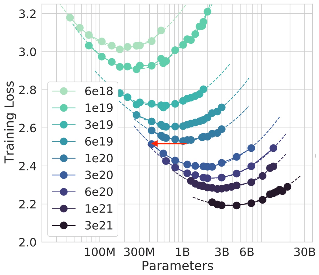
This gets you the same loss as before. You have to spend more compute during training, but in return, you get a smaller model that costs less compute at inference.

While this insight isn’t especially surprising, it took Meta releasing its LLaMA models in February 2023 to make it popular. By continuing to train models on even more data than Chinchilla implied, they were able to produce a 13B model that beat GPT-3 and a 65B model that beat Chinchilla.

Since then, subsequent LLaMA models like the LLaMA 3 series have gone even further. For a sense of scale, the 8B model was trained on 15T tokens. That is 75x the Chinchilla-optimal amount of 200B tokens for its size. This allowed it to match Chinchilla across a wide range of benchmarks, despite being an order of magnitude smaller.

What about inference?

It’s been four years since Kaplan first came out, and at this point, the core decisions in scaling up pretraining are pretty settled. While it’s hard to tell what the closed frontier labs are doing, the open-source researchers are broadly following the LLaMA recipe and producing models which are competitive with state-of-the-art closed-source models.

One key insight unlocked by the LLaMA models is that inference compute matters too, and you can trade off training compute and inference compute. What happens when we start to scale inference compute? Come back tomorrow to find out!

Thanks to Kevin Niechen, Zhengdong Wang, Jannik Schilling, Bradley Hsu and Devansh Pandey for discussion and feedback.